Electric-Gas-Heat Coordination
Energy hub scheduling with multiple energy networks
Electric-gas-heat network is a very common energy hub infrastructure in the microgrid (usually referred to as part of the future smart cities). They are co-related to each other since one type of energy could be easily converted to another, so a global scheduler or controller for these energy types is often warranted in the microgrid study. One might argue that a distributed control mechanism for each energy type might fit more with the distribution system since the decentralization is the main idea of adopting microgrid. However, it should be suggested that a central controller for the energy hub is more efficient considering the relatively small size of the problem and the concept of “fewer local bureaucratics”.
This project is funded by GEIRI-NA, which is currently closed due to Chinese local policies. We work closely with the former Senior Researcher Dr. Xiaohu Zhang, who is now the Principal Machine Learning Scientist at Plus Power and the former Research Director Dr. Di Shi, who is now an Associate Professor at New Mexico State University.
This research involves the co-simulation and scheduling of the generating units, energy storage systems (including all the electric, gas, and heat storage systems), and renewable assets from a distributed microgrid in the wholesale energy market operation. We need a comprehensive modeling of the triumvirate of electric, gas, and heat networks to fully capture the energy flow inside the energy hub. We will discuss them in details in the following sections.
Electric Network
In the electric network modeling, I used the DistFlow model (explained well in this post), which is commonly used in the operation and optimization of electrical distribution systems. It is a set of equations that describe the flow of power in a radial distribution network. It models the relationship between power injections, power flows, and voltages along the distribution lines.
\[v_{i,t}-v_{j,t}=\frac{r_{\ell}p_{\ell,t}+x_{\ell}q_{\ell,t}}{V_0},\]where \(v_{(i,j),t}\) denotes the voltage of bus \(i\) or \(j\) at timestep \(t\), \(r_{\ell}\) and \(x_{\ell}\) denote resistance and reactance of line \(\ell\) (connecting \(i\) and \(j\)), and \(p_{\ell,t}\) and \(q_{\ell,t}\) denote active and reactive power flow of line \(\ell\) at timestep \(t\). Using this equation together with capacity/voltage limit constraints and power balance equation, we could approximate the distribution-level power flow and thus model the network.
Gas Network
The gas network flow problem is highly nonlinear due to the notorious Weymouth equations. A common way to do this is to use the second-order cone program to convexify the nonlinearity.
\[(1-\alpha^c)u_{\ell,t}^{in} = u_{\ell,t}^{out},\] \[\omega_{j,t}\leq \gamma_c\cdot \omega_{i,t}\] \[u_{\ell,t}^2 \leq \theta\cdot(\omega_{i,t}^2-\omega_{j,t}^2),\]where \(\alpha_c/\gamma_c\) denote the gas/inflow compressor factors, \(\omega_{(i,j),t}\) denotes the gas nodal pressure of node \(i\) or \(j\) at timestep \(t\), \(u_{\ell,t}\) denotes the gas pipeline flow of pipeline \(\ell\) (connecting \(i\) and \(j\)) at timestep \(t\), and \(theta\) is the Weymouth coefficient. The second inequality formulates a second-order cone in the constraint space.
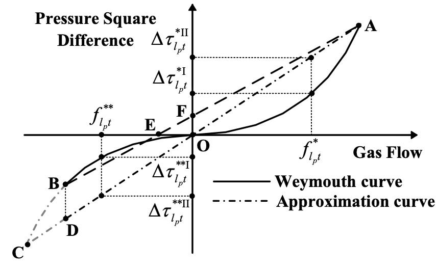
Alternatively, there is another way, which is far more straightforward, to actually linearize the Waymouth equation. The figure below depicts the overall idea of this linearization. The solid curve AC is the original Weymouth curve, and we use the dashed curve AC to approximate the accurate Weymouth curve. The accuracy of this approximation is guaranteed based on the assumption that the maximum allowable pressure of the initial node of the pipeline is no smaller than that of the terminal node. We also argue that the pressure lower bound of gas nodes are all the same, but the pressure upper bound of gas nodes are different, which creates an asymmetric line (AB). Thus, we make an extension to the third quadrant to make a symmetric line (AC).

Using this approximation, we render the linearized version of the Weymouth equation as below.
\[(1-\alpha^c)u_{\ell,t}^{in} = u_{\ell,t}^{out},\] \[\omega_{j,t}^2 \leq \gamma_c^2\cdot \omega_{i,t}^2 ,\] \[\omega_{i,t}^2 - \omega_{j,t}^2 = u_{\ell,t}\cdot \sqrt{\frac{\omega_{i,t}^{\max} - \omega_{j,t}^{\min}}{\theta}}.\]Heat Network
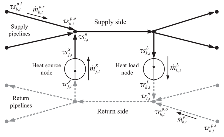
The heat network is also a very complicated energy network. The heat network consists of symmetric supply and return pipelines, and the figure below shows a typical topology of the heat system. At each source (load) node, heat is injected into (withdrawn from) the network via a heat exchanger between the supply side and the return side. The network model obeys the hydraulic conditions and thermal conditions.

Hydraulic conditions describe the continuity of mass flows. For each node, the mass flow entering the node is equal to the mass flow leaving the node.
\[\sum_{b \in S_i^{P, e}} m_{b, t}^{p, s}+\sum_{j \in S_i^S} m_{j, t}^S=\sum_{b \in S_i^{P, s}} m_{b, t}^{p, s}+\sum_{k \in S_i^L} m_{k, t}^L\] \[\sum_{b \in S_i^{P, e}} m_{b, t}^{p, r}+\sum_{j \in S_i^L} m_{j, t}^L=\sum_{b \in S_i^{P, s}} m_{b, t}^{p, r}+\sum_{k \in S_i^S} m_{k, t}^S\]We leave the notation at the end of this section. Thermal conditions characterize the relationship among nodal temperatures and thermal energy productions/consumptions, and consist of the following constraints. Thermal energy provided by the combined heat and power (CHP) unit is
\[h_{i, t}^S=c_p m_{i, t}^S\left(\tau s_{i, t}^S-\tau r_{i, t}^S\right)\]Heat consumption at a load node is
\[h_{i, t}^L=c_p m_{i, t}^L\left(\tau s_{i, t}^L-\tau r_{i, t}^L\right)\]Temperature at confluence nodes satisfy
\[\sum_{b \in S_i^{p, e}}\left(\tau s_{b, t}^{p, o} m_{b, t}^{p, s}\right)+\sum_{j \in S_i^S}\left(\tau s_{j, t}^S m_{j, t}^S\right)=\tau s_{i, t}^n\left(\sum_{b \in S_i^{p, e}} m_{b, t}^{p, s}+\sum_{j \in S_i^s} m_{j, t}^S\right)\] \[\sum_{b \in S_i^{P, s}}\left(\tau r_{b, t}^{p, o} m_{b, t}^{p, r}\right)+\sum_{k \in S_i^L}\left(\tau r_{k, t}^L m_{j, t}^S\right)=\tau s_{i, t}^n\left(\sum_{b \in S_i^{P, e}} m_{b, t}^{p, s}+\sum_{j \in S_i^S} m_{j, t}^S\right)\]Due to inevitable heat loss, the temperature of fluid in pipelines drops along the flow direction. The relationship between inlet and outlet temperatures of each pipeline is established as
\[\tau s_{b, t}^{p, o}=\left(\tau s_{b, t}^{p, i}-T_t^a\right) e^{\frac{\lambda_b L_b}{c_p m_{b, t}^{p s}}}+T_t^a\] \[\tau r_{b, t}^{p, o}=\left(\tau r_{b, t}^{p, i}-T_t^a\right) e^{\frac{\lambda_b L_b}{C_p m_{b, t}^{p, r}}}+T_t^a\]The heat loss in a pipeline is expressed as follows
\[\Delta Q_t^b=C_p m_{b, t}^p\left[\left(\tau_{b, t}^{p, i}-\tau_{b, t}^{p, o}\right)\right]\]Due to the bilinear and exponential nature in the above equations, the above model is nonlinear. Here, I use a heuristic method to approximate the nonlinear constraints. It is observed that when mass flow variables are fixed, the thermal constraints in the heat system become linear. The heuristic variable temperature constant flow (VT-CF) can determine the near-optimal mass flow rate (MFR) based on network loss analysis. To do so, we first substitute the above three equations to obtain
\[\Delta Q_t^b=C_p m_{b, t}^p\left[\left(\tau_{b, t}^{p, i}-\tau_{b, t}^{p, o}\right)\left(1-e^{-\frac{\lambda_b L_b}{C_p m_{b, t}^{p, \tau}}}\right)\right]\]where \(0<\frac{\lambda_b L_b}{c_p m_{b, t}^{p, r}} \ll 1\). Since \(e^{-x} \approx 1-x\), we have
\[\Delta Q_t^b=C_p m_{b, t}^p\left(\tau_{b, t}^{p, i}-T_t^a\right) \frac{\lambda_b L_b}{C_p m_{b, t}^{p, r}}=\lambda_b L_b\left(\tau_{b, t}^{p, i}-T_t^a\right)\]This equation suggests that \(\Delta Q_t^b\) is independent of MFR \(m_{b,t}^p\). Hence, by fixing MFR, the above heat system operation model is a linear program. Then, I use a heuristic two-step hydraulic-thermal decomposition to find a near-optimal solution with good quality. The workflow is summarized below.
- Step 1: Set all pipeline temperatures to the lower limits and calculate the heat loss.
- Step 2: Calculate the required heat sources by the summation of heat demand and the calculated heat loss. Then calculate the heat source and heat load MFR per their models.
- Step 3: Calculate the pipeline MFR per the MFR balance equations.
- Step 4: Fix all MFR variables, then perform the optimization.
The following table provides all the notations throughout this subsection.
| Variables | Notations |
|---|---|
| \(p_{h,t}\) | Power produced from CHP unit \(h\) at timestep \(t\) |
| \(h_{h,t}\) | Heat energy produced from CHP unit \(h\) at timestep \(t\) |
| \(m_{b, t}^{p, s} / m_{b, t}^{p, r}\) | Mass flow rate in supply/return pipeline |
| \(m_{i, t}^S / m_{i, t}^L\) | Mass flow rate in heat source/load |
| \(\tau r_{b, t}^{p, i} / \tau r_{b, t}^{p, o}\) | Temperature at inlet/outlet of the return pipeline |
| \(\tau s_{b, t}^{p, i} / \tau S_{b, t}^{p, o}\) | Temperature at inlet/outlet of the supply pipeline |
| \(\tau s_{i, t}^S / \tau s_{i, t}^S\) | Supply/return temperature of heat source |
| \(\tau s_{b, t}^L / \tau r_{b, t}^L\) | Supply/return temperature of heat load |
| \(\tau s_{i, t}^n / \tau r_{i, t}^n\) | Mixture temperature at supply/return node |
| Parameters | Notations |
|---|---|
| \(C_p\) | Specific heat capacity of water |
| \(h_{i,t}^{L}\) | Energy demand of heat load |
| \(L_b\) | Length of pipeline |
| \(T^a_t\) | Ambient temperature at timestep \(t\) |
| \(\lambda_b\) | Heat transfer coefficient of pipeline |
After modeling all the electric, gas, and heat networks, I added generating unit modeling and energy storage system modeling for all energy types, then performed the simulation on multiple scenarios to confirm the efficacy of the proposed model.
Further Works
I further extend this research to a transmission and distribution system coordination problem considering the uncertainties brought in the microgrid since abundant wind and solar energy are in the local energy hub. I leveraged the distributionally robust optimization to account for those uncertainties while devising a novel ADMM-like algorithm to efficiently solve it. Interested readers could refer to this paper.