startup/shutdown prediction

This project was the main contribution I devoted when I was co-op with MISO. We collaborated with Dr. Junshan Zhang from ASU (now with UC Davis), Dr. Ben Knueven from NREL, Dr. Manuel Garcia from Sandia Lab, and Dr. Roger Treinen from Nexant. Here is a mid-term report submitted to ARPA-E.

Generation uncertainties, especially during the unit startup and shutdown (SU/SD) processes, pose uncertainties for the real-time market clearing process, and they are often underestimated. We propose two approaches to predict generator SU/SD trajectories in the real-time operations. We first collect and pre-process raw market data from state estimation. Then we investigate two approaches to account for the uncertainty in MW of generation SU/SD in the real-time market clearing. The first is an offline approach that leverages gradient boosting tree (GBT) to effectively capture the nonlinear relationship between the SU/SD curves and selected feature maps. The offline approach works for predicting generator trajectories in the real-time Look Ahead Commitment (LAC) process based on historical data. We also investigate an online approach using a long-short-term memory network (LSTM) that can learn from the last-interval error information and enhance the current prediction, potentially applicable for the real-time economic dispatch process, which is called Unit Dispatch System (UDS) at MISO. We validate the benefit of the proposed approach with a full-day rolling LAC framework on MISO-size test cases. The result shows that using the predicted curves could help system operators achieve better results in real-time commitment and dispatch processes.

My work was focusing on developing the two predictive approaches using GBT and LSTM. But firstly, as “garbage-in garbage-out”, what needs to be done at the beginning is the data preprocessing, including data mining, cleaning, and potential augmentations.

Data Preprocessing

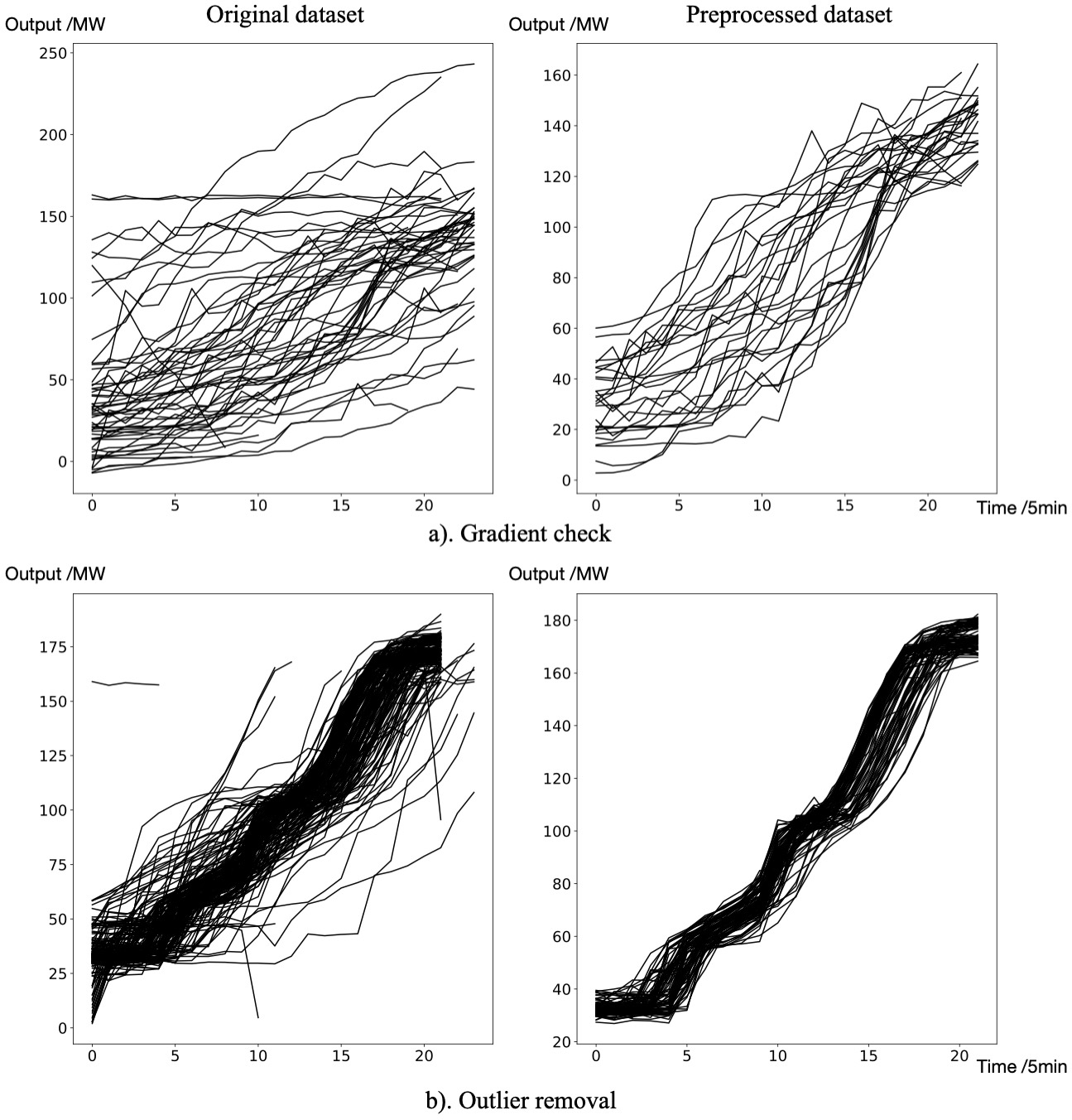
The raw data in the system operators’ database comes from the transmission state estimation and contains many noise and error measurements. The overall preprocessing steps are as follows:

• Query the raw timeseries data from the database. As LAC has a three-hour horizon, we consider SU/SD curves within two hours. Based on the industry practice, for SU/SD predictions, we use the two hours before the startup effective time for the startup prediction and two hours after the shutdown signal is sent, respectively. Hence, each raw timeseries instance has a maximum of 24 intervals with a five-minute resolution.
• Check the gradient of the curve. For a startup timeseries, if it has more than half consecutive negative gradients, or its curve gradient is too small for all intervals, it will be deemed a wrong measurement and removed. For the shutdown timeseries similar logic is applied.
• Remove the outliers using the interquartile range method. In our study, we generally set \(Q_1=0.25\) and \(Q_2=0.75\) (see the following equations). We also remove all duplicate measurements in this step.

• For missing measurements in one timestamp, we impute with the median of neighborhoods. For instances with more than half missing measurements, we remove these instances.
• If 90% timeseries instances of one unit could reach the minimum power output within five/fifteen minutes, the unit is excluded from the startup curve prediction for UDS/LAC, respectively. For the shutdown timeseries we apply similar logic.

By following this procedure, here is one sample preprocessing:

Feature Selection

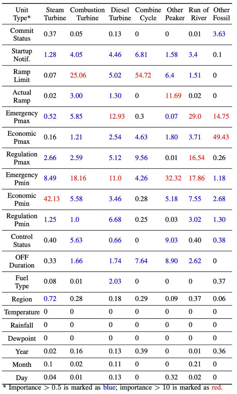
After the data preprocessing is complete, we conduct feature selection by applying the Deep Feature Synthesis algorithm. This algorithm follows the inherent relationships between original input features and then sequentially applies mathematical functions along the relationships to create new features. It is efficient when we do not know the complete list of correlated features. More details about how to implement this algorithm can be found here.

The final feature scoring for different types of units based on the feature selection procedure is as follows:

Gradient Boosting Tree: Offline Predicting

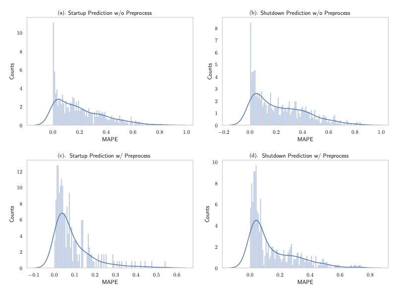
Gradient boosting tree (GBT) is a boosting algorithm using ensembled decision trees. By leveraging the greedy boosting concept, stage-wise decision trees use the last-stage prediction residuals as training data to enhance the initial prediction, reducing both the bias and variance. However, we have lots of categorical features in our problem, which could not be directly applied with GBT. Hence, we leverage the categorical boosting algorithm with Catboost to perform our prediction. We use around 1,000 generating units with different types in our analysis. The test MAPE for each unit is shown below, compared between the preprocessed datasets and raw datasets. Certainly, the dataset is divided into a training set (75%) and a testing set (25%).

Long-Short-Term Network: Online Predicting

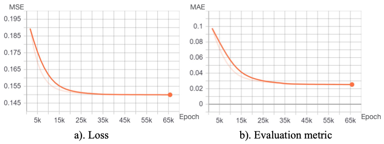
While the offline approach suits the need of the LAC curves, for real-time UDS with finer granularity, the prediction quality of the offline approach needs further improvement. However, the UDS follows a rolling-horizon manner, which means for every five minutes, we could leverage the previously predicted error to enhance the current-interval prediction. This asynchronous error correction could be best tackled by an LSTM network. We adopt the following LSTM framework:

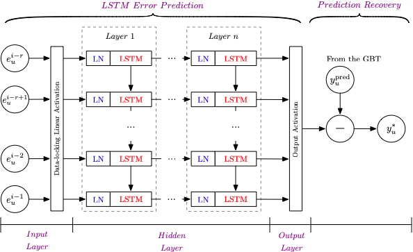
Each LSTM cell leverages layer normalization (LN) to smooth the activations along the feature direction with whitening. The training procedure observed from TensorBoard is as follows:

Economic Assessment

After we obtain the startup/shutdown curves discussed above, we plug in these curves for the LAC and UDS coordinated operation. We studied all units recorded in the MISO state estimation for the startup/shutdown curve prediction, but not all generators within the operation have associated curves. Some units might have startup/shutdown time shorter than fifteen minutes, while some units are not frequently committed or de-committed. We choose units with a high prediction performance of startup/shutdown curves, i.e., MAPE less than 10%, in the test case. Whole-day operations with the rolling LAC instances and associated UDS instances are executed for a sample week in this study. Using SLAC could better capture the system characteristics conditioned by the uncertain renewable resources. Then, we pick two days, i.e., Day 1 and Day 5, to see whether the predicted startup/shutdown curves could synergize with SLAC. Below shows the economic improvements:

It is clear from the row of LAC + Curves that using the curves in LAC contributes to overall cost reduction. Only Day 2 has an increase of production cost using the curves, but it achieves the highest penalty reduction among all days. Note that, though the percentage reduction seems tiny, the base value is with the magnitude of tens of millions of dollars. Hence, capturing the startup/shutdown uncertainties in the current real-time market clearing process holds the potential to help the operator achieve better market-clearing results and reduce unnecessary penalties of violations. It is also interesting to find that using the predicted curves helps SLAC further reduce the production cost and penalty cost compared with the deterministic LAC. Using startup/shutdown curves makes committing/de-committing units yield more accurate economic schedules, strengthening SLAC’s capability of handling different system scenarios. Note that all the numbers here, though seems small in percentage, indicates levels of millions of dollars saving in the daily operation. Hence in fact, the improvement of using the proposed approach could practically save a lot in the every day’s scheduling.