MIDAS-Scheduling

MIDAS-Scheduling is the first open-source Python package I developed for creating an academic equivalent to commercial energy market simulation software (they cost a lot!) like PLEXOS and Aurora. Researchers from NREL previously developed a similar-use software based on MATLAB called FESTIV, but MATLAB is not a free software as well. MIDAS-Scheduling leverages open-source packages such as Numpy, Pandas, and Pyomo to build the optimization model for market operations. We extensively focus on unit commitment and economic dispatch and their inter-correlated timestep wrapping. Needless to say, most unit modules, to the best of implementability, have been included in the consideration. Models for thermal, hydro, battery, nuclear, and gas units are handy to use, together with their unique but complete representations of ancillary service provisions.

Unfortunately, this package is now under control by NREL, and the release date is undetermined. The project PI was Dr. Jin Tan, while the major collaborators with NREL were Dr. Xin Fang (now with Mississippi State University) and Dr. Harry Yuan (now with Entergrid, LLC).

As this is the first open-source package I developed, the coding style was not well regularized and the performance was not optimized. NREL used this package to work for a DOE SETO-funded project called MIDAS-Solar. It developed both a multi-timescale grid simulation model and an integrated photovoltaic (PV) model to seamlessly simulate solar PV variability and its impact on power system operations from economic scheduling timescales (day-ahead to hours) to dynamic response analysis (seconds to sub-seconds). For scheduling with very high levels of inverter-based resources (IBRs), up to and including 100%, stability of grid controls was evaluated through targeted electromagnetic transient (EMT) simulations and power hardware-in-the-loop simulations of key transient events at key schedule points. NREL has a detailed description page to disseminate this.

My work was focusing on developing the MIDAS-Scheduling package and all the other stuffs NREL did were still conducted via commercial software like PSSE and PSCAD. Due to proprietary information limit, I could not say much about the details for MIDAS-Solar.

Here is the framework for MIDAS-Scheduling:

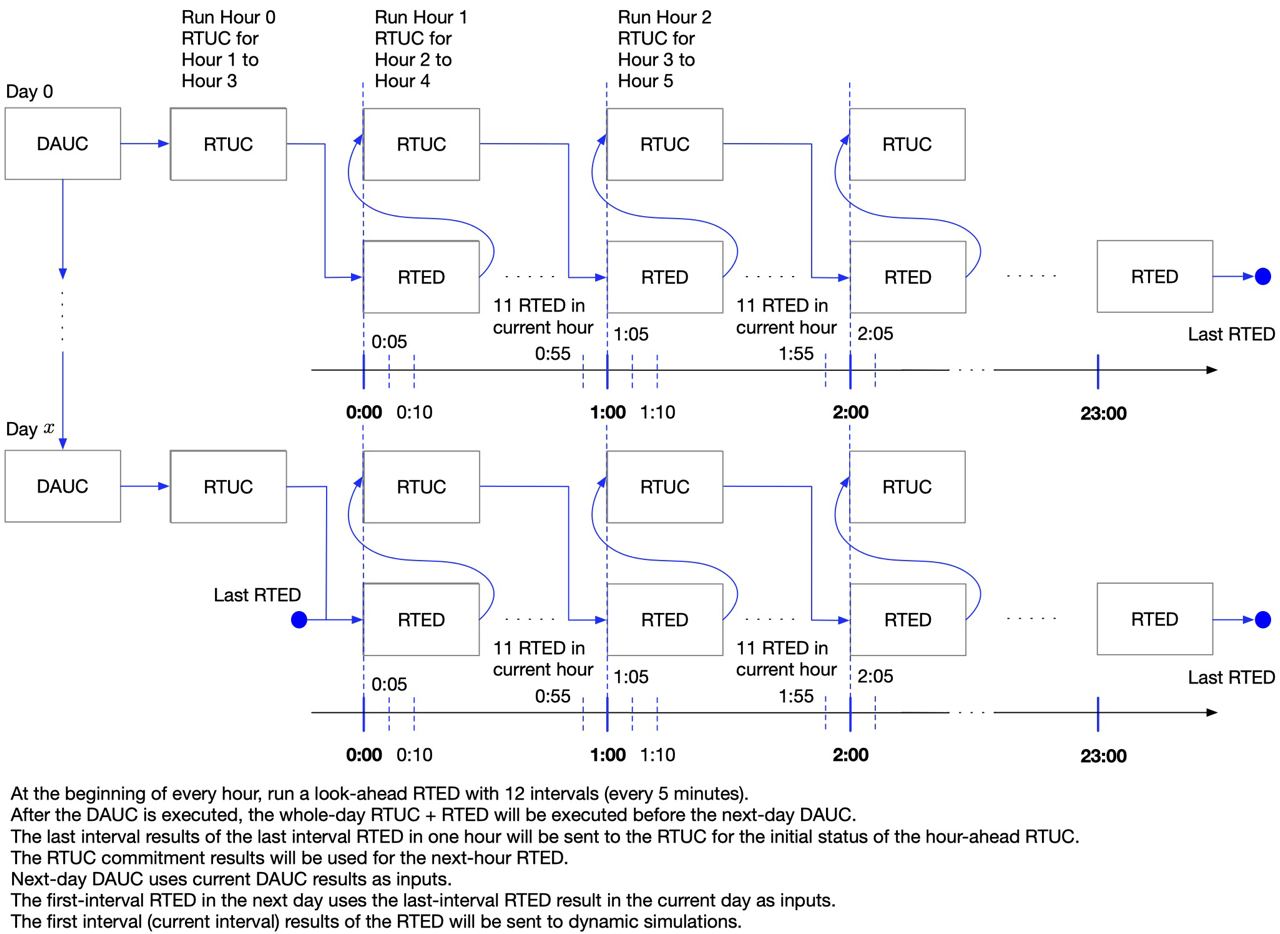
MIDAS-Scheduling integrates four sub-modules: day-ahead unit commitment (DAUC); day-ahead economic dispatch (DAED); real-Time unit commitment (RTUC); real-time economic dispatch (RTED). Each sub-module could have different timescales exercising system operation practice. Through the simulation on MIDAS-Scheduling, users can test with changing the input scenarios and PV power plant control strategies to study the impacts of these changes on the system-wise economics, reliability, and stability of the system, especially for cases with high PV energy penetrations.

During the simulation, the DAUC, RTUC, and RTED submodules will have the major interaction. The major function of DAED sub-module is to receive the unit-commitment results from DAUC and calculate day-ahead LMP to decide the DA generation schedule. The commitment results of DAUC will be applied to the RTUC and RTED submodules and the flexible units can adjust their commitment status in RTUC as well.

The formulations of four sub-modules are similar. The objective functions in all sub-modules are to minimize cost include generation cost to serve the load including the start-up cost in the commitment, ancillary service cost, load-shedding cost, ancillary service penalty cost, and some constraints violation penalty costs. However, the DAUC and RTUC sub-modules can determined the on/off status for all generators but the DAED and RTED sub-module only can determine the power dispatch on each generation unit. Another major difference is the time resolution of sub-modules. In general the time resolution of DAUC is 1 hour, and the predict horizon is 24 hours for the study day plus additional 2 hours of the day following the study day for the purpose of continuity of commitment; the DAED time horizon and resolution are the same with the DAUC; the time resolution in RTUC is 1 hour, and the predict horizon is 3 hours; the time resolution of RTED is 5 mins, the predict horizon is 2 hours.

More details regarding the software like necessarily dependent packages and virtual environment setups could refer to the MIDAS-Scheduling documentation (not release yet 😴). It utilizes CSV as data I/O. It is recognized that CSV processing is inefficient but we deem it is sufficient for the energy market transaction volume. We also have handy utility functions for users to calculate the transmission sensitivity matrices like PTDF and LMP.

I’d like to introduce more about some fun stuffs of MIDAS-Scheduling.

Storage Modeling

In detail, we consider an energy storage system (ESS) with a general and flexible setting. The ESSs incorporated in our system can have flexible types, including pumped storage and battery storage. For the storage simulation modeling, we consider the idle status of the ESS unit, and whenever it is charging, discharging, or idle, it can provide ancillary services (ASs) in both up and down directions. This is the key advantage of our schemes compared with the SOTAs. Our ESS framework can fully leverage the ESS’s flexibility for both energy and ASs and better contribute to the system scheduling operation, particularly with PV units.

As shown above, the pumped storage (PESS) can provide both up and down services in the three states, while the battery storage (BESS) can provide ASs under a more flexible setting that honors the fact that the battery storage can respond much faster. The system operators can more explicitly consider ESSs’ two types of flexibilities in the market operation, which can yield more practical and accurate decisions. Read more details in our NAPS paper.

Startup/Shutdown Trajectories

In real world, synchronous generators require start-up time and shutdown time to perform turn-on and turn-off. We differentiate generators by their trajectory time to flexible units, inflexible units and renewable units. The inflexible units’ trajectories are modeled in the DAUC, and the flexible units’ trajectories are modeled in the RTUC. Certainly, during startup/shutdown trajectory, the generator cannot provide any ancillary service (excluding non-spinning reserve capacity).

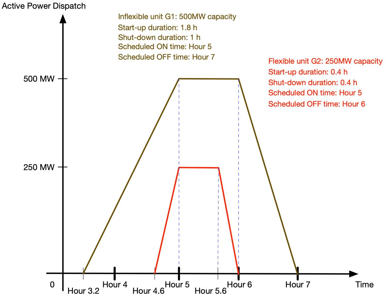
Say, if Unit G1 is scheduled to startup at Hour 5, in the real-time operation, considering its startup time, the unit will be actually started at Hour 3.2, as the scheduled startup at Hour 5 means it should be at least reaching its minimum capacity at that time. Conversely, for shutdown, if Unit 1 is scheduled to shutdown at Hour 6, it will actually begin its shutdown at Hour 6 in real time, because practically that is the moment when the unit receives the shutdown signal.

Fixed-interval RTUC

Since RTUC is also a rolling-horizon operation, the operator will update the startup/shutdown statuses in the most recent RTUC. Hence, if the current RTUC changes the startup decision determined in the last RTUC, the non-spinning reserve scheduled in the last RTUC will violate the startup logic. Hence, we develop the following scheme: the first interval’s commitment is fixed by the second interval’s commitment in the last RTUC. The first interval’s commitment of each RTUC is consistent in any connecting period and hence will not violate the last RTUC’s startup decisions.

Note that this scheme has been actually adopted by MISO, a famous ISO in the U.S.

Some showcases of the result output

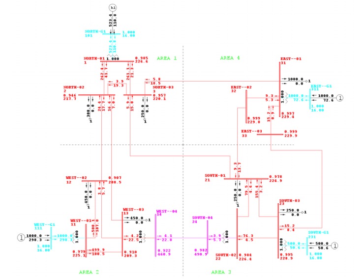
We use the toy 18-bus system reduced from the WECC system as an example. Here is the diagram:

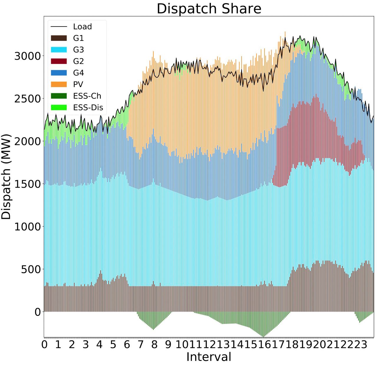
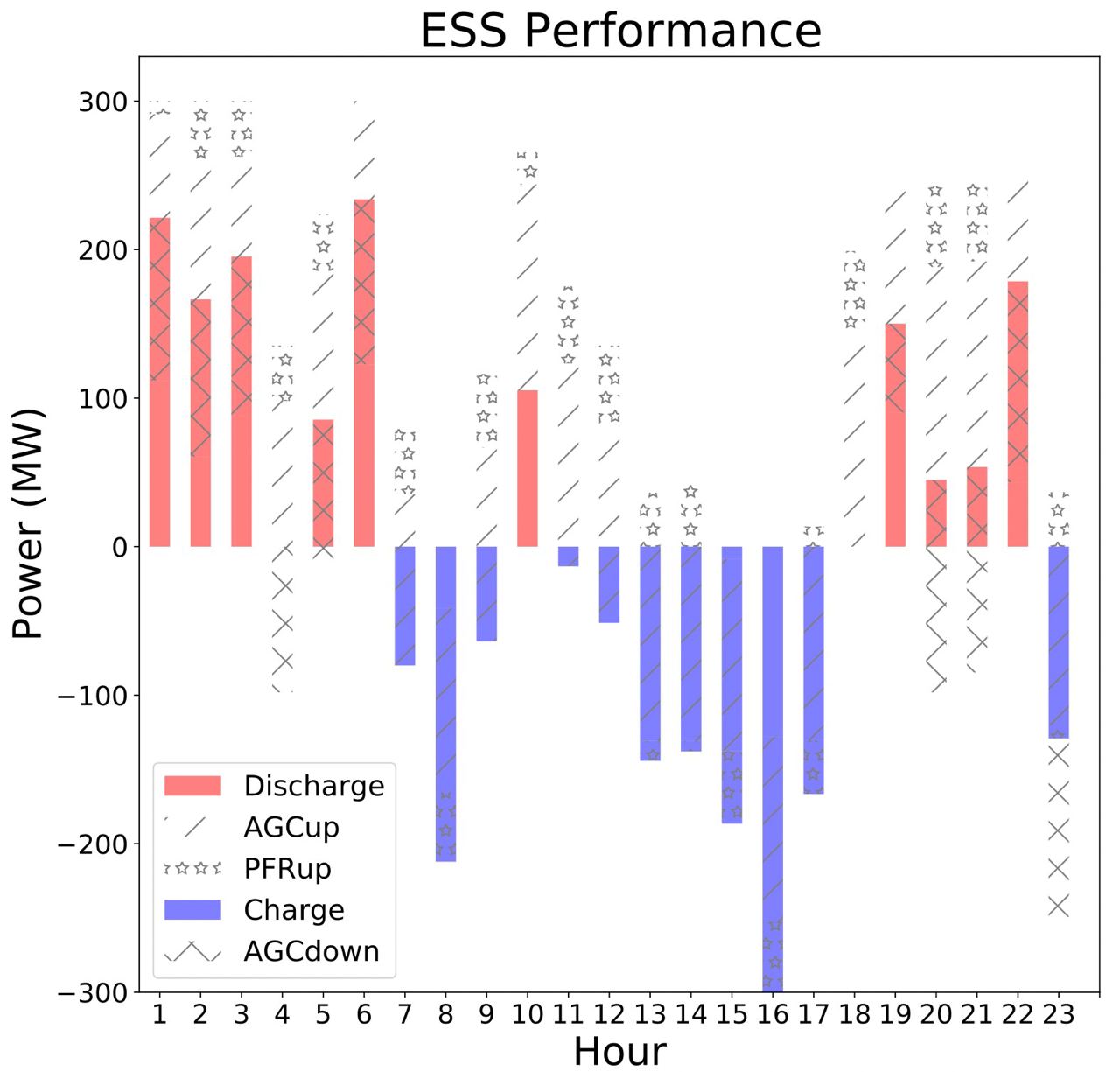
After running the MIDAS-Scheduling program, the automated result-generation code will provide you with the following fancy-looking summary charts:

Some showcases of the code snippets

If you are interested in how I structure the code, here is how users run MIDAS-Scheduling interactively:

import midass as ms

results_mode1 = ms.run_mode1(solver_name = "gurobi",
                             prefix_dir = r"midass/data/18_bus/",
                             verbose = True)
results_mode4 = ms.run_mode4(solver_name = "gurobi",
                             prefix_dir = r"midass/data/18_bus/",
                             psse_folder = r"PSSE/",
                             case_name = r"Case1",
                             run_name = r"Case1_24hr",
                             close_loop_flag = False, 
                             ess_interpolate_method = True,
                             ess_dispatchable = False, 
                             verbose = True)

Fig_Plot = ms.FigurePlot("DAUC",  results_mode4)

Here is how we build the DAUC model inside the code:

UCmdl = pe.AbstractModel()
Params.DAUC_read_params(UCmdl)
Vars_base.load_base_vars(UCmdl)

getattr(Vars_gen_power, "DAUC_Piecewise_power")(UCmdl)
getattr(Vars_ess_power, "Idle_2var_power_soc")(UCmdl)

getattr(Constr_gen_ancillary_service, "DAUC_AS")(UCmdl)
getattr(Constr_ess_ancillary_service, "DAUC_AS")(UCmdl)

getattr(Constr_power_balance, "Nodal_power_balance")(UCmdl)
getattr(Constr_sys_reserve, "AS_Coupled")(UCmdl)

getattr(Objective_function, "DAUC_objective_basic")(UCmdl)

Here is how we define constraints inside the model:

def _Define_PFRup(md):

    def pfr_pos_cap_rule(md, gi, hi):
        return md.gen_pfr_pos[gi,hi] <= (md.Df_Max - md.Gen_DB[gi]) / md.Gen_Ri[gi]
        
    md.gen_pfr_pos_cap = pe.Constraint(md.DPGEN_SET, md.INTER_SET, rule = pfr_pos_cap_rule)
    
@add_model_attr(component_name, requires = {'params_loader': None,
                                            'base_var_loader': None,
                                            'power_var_loader': None,
})

def DAUC_AS(md):
    
    _Define_PFRup(md)

Hope NREL could release the software soon, and have fun running your cases using MIDAS-Scheduling! I’m open to any consulting service and software support. Contact me for pricing.